This guided example is a supplement to the more general chapter offering a framework and workflow for power analyses. It follows the general steps outlined there. In this example, we will use the package brms for Bayesian estimation of parameter values. To keep things computationally tractable, we will focus on a simple comparison between two independent samples. The general steps are applicable to other Bayesian designs.
Pre-requisite: You will need to set up RStan on your computer for the Bayesian analyses in this example to work. See mc-stan.org and Rstan’s wiki.
David Reinstein on installation on a Mac
I never managed to install “mac -os Rtoolchain” but I did manage to get #Rstan up and running thanks to the Coatless Professor’s workaround.
2 Step 1: Generate a large number of data sets for the analysis
We will run a comparison of two independent samples, and seek to assess our capacity to detect 1 a range of possible effect sizes, considering Cohen’s \(d\) at 0, .15, .3.
Code
#We will also increase the memory limit in R to allow for the large objects that are likely to be created:memory.limit(100000)
[1] Inf
Code
#This is a Windows specific function. Some possible ways to do this in Mac are suggested here: https://stackoverflow.com/questions/51295402/r-on-macos-error-vector-memory-exhausted-limit-reached
The code t.data.maker below
Creates a dataframe with two groups
each with the same group.size (easy to adjust this to allow 2 sizes)
each drawn from standard normal distribution
group b’s mean differs from group a according to the specified effect.size
sim is just the counter of ‘which simulation this is’
one row per ‘observation in group’… so 2*group.size rows
Code
#| label: data-making-function#| code-summary: "function to make simulated data"t.data.maker <-function(sim, effect.size, group.size) {# create a data frame with two groups, standard normal distribution# group b differs from group a according to the specified effect size data <-tibble(a.group =rnorm(n = group.size, mean =0, sd =1), #create `group.size` rows of a standard normal,b.group =rnorm(n = group.size, mean = effect.size, sd =1), #... of a std normal shifted by `effect` for 'treatment group' (or after-treatment if this is within subject)n =seq(1:group.size), #counter'effect.size'= effect.size,'sim'= sim ) %>%pivot_longer(cols = a.group:b.group, #make this one row per 'observation in group' (rather than 1 per observation with 'both groups') ... so 2*group.size rowsnames_to ='group',values_to ='response')return(data)}
We will run 250 analyses2 for each of the three effect sizes of interest. We use maximum group sizes of 1500.3 We put these into a format to pass to a map function, and then run the data-making function over the different effect sizes to generate the many data sets.
In the code below, we create this simulated data, creating a list of tibbles, one tibble for each simulated data set, considering the three effect sizes.
iterate-datamaker
# set up furrr to run iterations more quickly ... this is (optional) parallel processing stufflibrary(furrr)plan(multisession)options <-furrr_options(seed =1234)# make a tibble with our intended effect sizes (DR: for 250 simulations each) effect.sizes <-tibble(effect.size =c(rep(0, 250), rep(.15, 250), rep(.3, 250)),sim =seq(1:750) )# run t.data.maker over all the requested data sets# Map the list of effect sizes (and sim counter) to `t.data.maker`#... to generate a list of tibbles (each of size 1500)#... as specified, with 250 'treated' and 250 'controls' per effect size, where controls are standard normal and treated have the given effect sizessim.data <-future_map2_dfr(.x = effect.sizes$sim,.y = effect.sizes$effect.size,.f = t.data.maker,group.size =1500,.options = options)# split the simulated data sets (into a list of tibbles, one tibble per simulation) for analysissim.data <- sim.data %>%group_by(sim) %>%group_split()
3 Step 2: Run the proposed analysis over the many data sets and return the estimands of interest
We set up a Bayesian regression model to run over the many simulated data sets.
Make sure this produces and saves your estimands!
It is important to ensure that the estimands we are interested in can be returned at this step, because this process can be time consuming. We don’t want to have to repeated it due to small mistakes. Hence, first carefully check that the code returns all the parameters you need, and then put it into a function that runs over the many data sets.
In any case, we need to run the model at least once outside of the function.4 This regression serves to compile the code and prevent the need to recompile it each time a new analysis is run, saving a lot of time.
Our simple formula for the t-test is a simple linear model:
Code
reg.form <- response ~1+ group
In the code below, we consider the nature of priors we can set for this model. We pass brms::get_prior our data, the family of response and link we want to use in the model, and the formula we are fitting. It suggests some possible priors or things to assign priors over?]
We aim for ‘weakly informative priors’, to constrain the model from entertaining highly unlikely parameter estimates. Setting reasonable priors on a model also helps speed up the MCMC sampling.
Code
# load in requisite packageslibrary(brms)library(tidybayes)# check what priors can be defined in the modelget_prior(formula = reg.form,data = sim.data[[501]],family =gaussian())
                  prior     class         coef group resp dpar nlpar lb ub
                 (flat)         b
                 (flat)         b groupb.group
 student_t(3, 0.2, 2.5) Intercept
   student_t(3, 0, 2.5)     sigma                                     0
       source
      default
 (vectorized)
      default
      default
# set our own priors( reg.prior <-c(set_prior("normal(0 , 1)", class ="Intercept"),set_prior("normal(0 , .8)", class ="b", coef ="groupb.group"),set_prior("normal(1, 1)", class ="sigma")))
          prior     class         coef group resp dpar nlpar   lb   ub source
  normal(0 , 1) Intercept                                    <NA> <NA>   user
 normal(0 , .8)         b groupb.group                       <NA> <NA>   user
   normal(1, 1)     sigma                                    <NA> <NA>   user
A normal with mean 0 and variance 0.8 over the group-b adjustment
A normal(1,1) over the standard error of the outcome (?)
Now we want to check that the model runs properly, and that we can extract the estimands of interest. We run the regression with the brm() command, and we extract and manipulate the estimands of interest by pulling out the posterior distribution from the model with posterior_samples():
Code
# grab a test data set from the many data setstest.data <- sim.data[[501]]# run the regression modelbase.reg <-brm(formula = reg.form,data = test.data,family =gaussian(),chains =2,cores =2,iter =1200,warmup =200,prior = reg.prior)(base.reg)
 Family: gaussian
  Links: mu = identity; sigma = identity
Formula: response ~ 1 + group
   Data: test.data (Number of observations: 3000)
  Draws: 2 chains, each with iter = 1200; warmup = 200; thin = 1;
         total post-warmup draws = 2000

Population-Level Effects:
             Estimate Est.Error l-95% CI u-95% CI Rhat Bulk_ESS Tail_ESS
Intercept        0.01      0.03    -0.04     0.06 1.00     1732     1459
groupb.group     0.30      0.04     0.23     0.37 1.00     1457     1362

Family Specific Parameters:
      Estimate Est.Error l-95% CI u-95% CI Rhat Bulk_ESS Tail_ESS
sigma     1.00      0.01     0.98     1.03 1.00     1894     1610

Draws were sampled using sampling(NUTS). For each parameter, Bulk_ESS
and Tail_ESS are effective sample size measures, and Rhat is the potential
scale reduction factor on split chains (at convergence, Rhat = 1).
Code
posterior <-as_tibble(posterior_samples(base.reg)) %>%# I use the names of the posterior sample columns# to calculate group means and Cohen's dmutate(a.group =`b_Intercept`,b.group =`b_Intercept`+`b_groupb.group`,d =`b_groupb.group`/ sigma)(posterior)
We can see that our model run smoothly (decent effect sample sizes, Rhat of 1), and that we can return the parameters of interest. This approach can apply to essentially any Bayesian model - all one needs to do is know which part (or parts) of the posterior they are interested in and extract it. We can now move on to running the analysis over the many data sets. On my computer, this set of analyses took about 10 minutes to complete. (3 Feb 2023 update – seems faster now)
Code
reg.maker <-function(simulated.data, base.reg = base.reg,breaks =seq(from =100, to =1500, by =100)) { data <- simulated.data# this function allows the sample size to be cut# so that we can see power for many different sample sizes cut.samples <-function(break.point, data) { cut.data <-filter(data, n <= break.point) cut.data <-mutate(cut.data,sample.size = break.point)return(cut.data) } data.cuts <-map_dfr(.x = breaks, .f = cut.samples, data = data) data.cuts <- data.cuts %>%group_by(sample.size) %>%group_split()# this function runs the regression model over the different sample sizes run.reg <-function(data, base.reg) { set.seed =as.numeric(data[1 , "sim"])# note use of the 'update' function rather than brm# to prevent need to recompile the model output <-update(base.reg,newdata = data,chains =1,cores =1,iter =1750,warmup =250) output <-as_tibble(posterior_samples(output)) output <-mutate(output,sample.size =nrow(data) /2,effect.size =pull(data[1, "effect.size"]),sim =pull(data[1, "sim"]),a.group =`b_Intercept`,b.group =`b_Intercept`+`b_groupb.group`,cohen.d =`b_groupb.group`/`sigma`)return(output) } samples <-map_df(.x = data.cuts, .f = run.reg, base.reg = base.reg)return(samples)}t1 <-Sys.time()regression.samples <-future_map_dfr(.x = sim.data,.f = reg.maker,base.reg = base.reg,.options = options)t2 <-Sys.time()t2 - t1head(regression.samples)
4 Step 3: Summarise the output returned in Step 2 to determine likelihood of achieving various inferential goals
The regression.samples object now contains posterior distributions for analyses of various effect sizes and sample sizes. For this example, our key outcome of interest is the effect size, measured as Cohen’s d. We can use the posterior distribution for Cohen’s d to draw various inferences about it. Some examples of possible ‘tests’ one might like to do with regards to a posterior distribution are presented below.
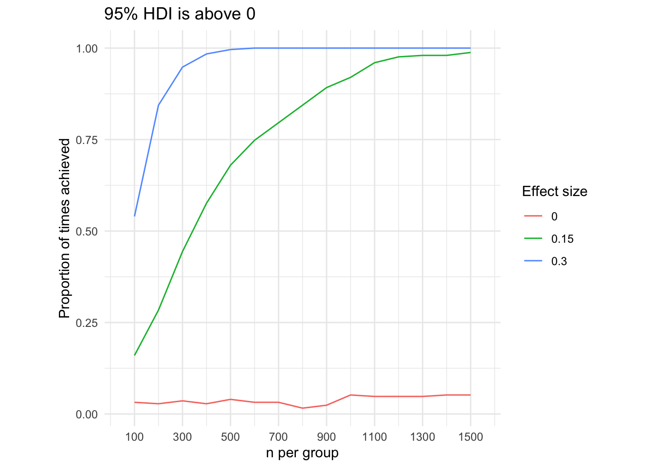
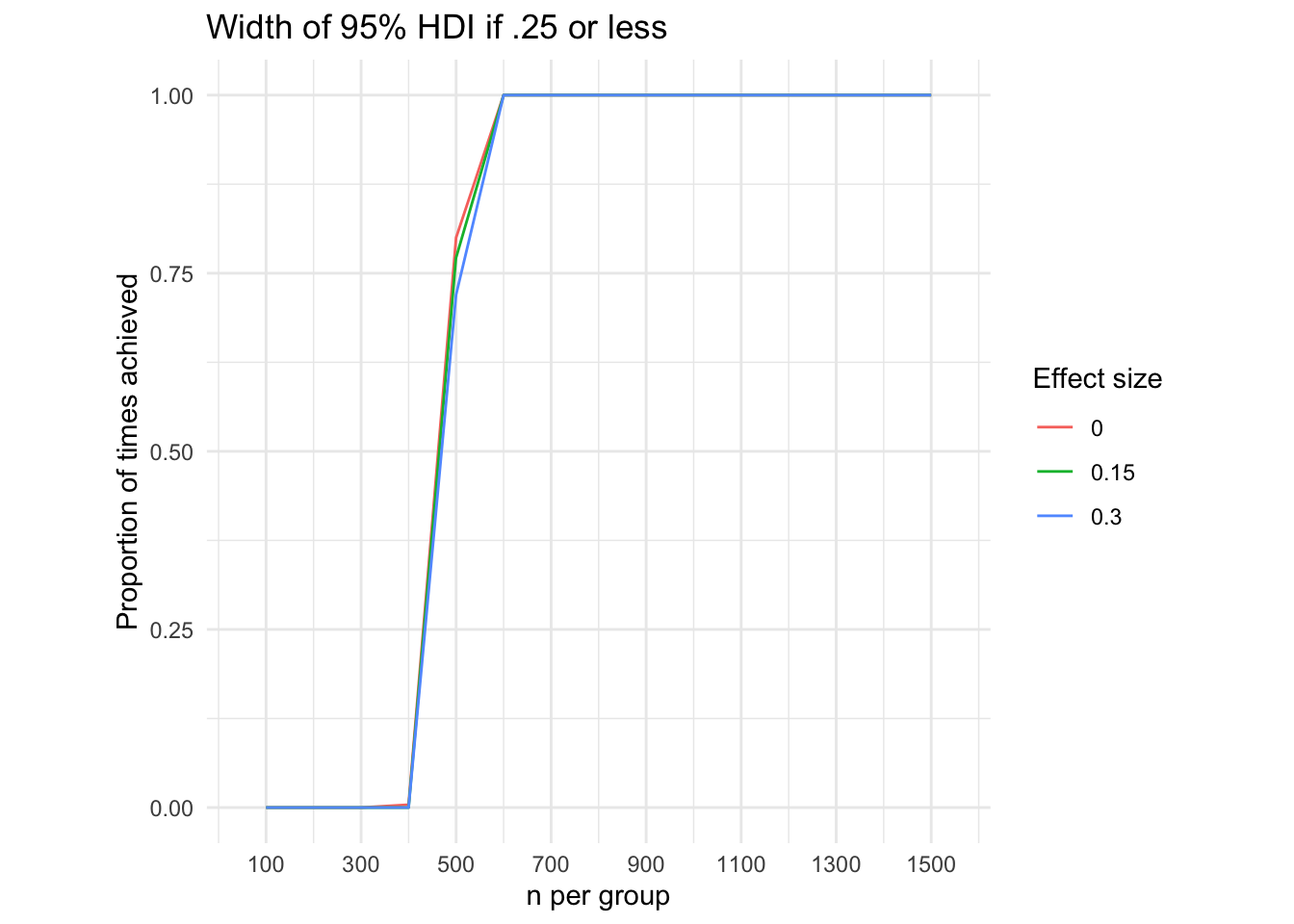
For the purposes of demonstration, we will focus on two possible metrics of interest. The first would be that the 95% Highest Density Interval (HDI: the 95% most probable values from the posterior) for Cohen’s d is greater than 0 (this is somewhat like a two sided t-test), and the degree to which we achieve a certain level of precision in the posterior estimate for Cohen’s d.
To do this, we simply need to make a function that will take each analysis (each posterior distribution for a particular simulation, sample size, and effect size), and determine the number of times across simulations that the posterior for Cohen’s d meets our decision criteria.
Code
# first split the posterior output according to sample size, effect size, and simulationregression.samples.split <-regression.samples %>%group_by(effect.size, sample.size, sim) %>%group_split()# make a function to summarise the posteriorposterior.inference <-function(posterior) {# take the posterior and retrieve the upper and lower# 95% hdi bounds for the effect size summary <- dplyr::summarise(posterior,lower95 =hdi(cohen.d, .95)[1],upper95 =hdi(cohen.d, .95)[2])# determine the width of the hdi and whether it is above 0# and add in meta information summary <-mutate(summary,width =abs(lower95 - upper95),width.25 =case_when(width <= .25~1,TRUE~0),above.0 =case_when(lower95 >0~1,TRUE~0),sample.size = posterior[[1, 'sample.size']],effect.size = posterior[[1, 'effect.size']],sim = posterior[[1, 'sim']])return(summary)}# feed the different posteriors to the summariserposterior.inferences <-future_map_dfr(.x = regression.samples.split,.f = posterior.inference, .options = options)
We can now count and plot the proportion of times we achieve our inference goals, according to different effect sizes, sample sizes, and goals. Note that in the case of determining whether the 95% HDI for Cohen’s d is above 0, the line for the effect size of 0 represents a false positive rate (because the effect size is in fact not above 0).
Code
above0 <- posterior.inferences %>%group_by(sample.size, effect.size) %>%summarise(.groups ='keep',n =sum(above.0)) %>%mutate('Proportion of times achieved'= n/250)precision25 <- posterior.inferences %>%group_by(sample.size, effect.size) %>%summarise(.groups ='keep',n =sum(width.25)) %>%mutate('Proportion of times achieved'= n/250)ggplot(data = above0) +scale_x_continuous(limits =c(50, 1550), breaks =seq(from =100, to =1500, by =200)) +geom_path(aes(x = sample.size, color =as.factor(effect.size),group =as.factor(effect.size), y =`Proportion of times achieved`)) +labs(x ='n per group', color ='Effect size', title ='95% HDI is above 0') +theme_minimal() +theme(aspect.ratio =1)
Code
ggplot(data = precision25) +scale_x_continuous(limits =c(50, 1550), breaks =seq(from =100, to =1500, by =200)) +geom_path(aes(x = sample.size, color =as.factor(effect.size),group =as.factor(effect.size), y =`Proportion of times achieved`)) +labs(x ='n per group', color ='Effect size', title ='Width of 95% HDI if .25 or less') +theme_minimal() +theme(aspect.ratio =1)
Note that, as would be expected, the chance that we achieve our goal of rejecting a non-zero effect varies with the true effect size. When we consider the precision of our estimates, the actual effect size is not relevant: the more data we gather, the more precise our estimates become, irrespective of the size true effect.7
DR: Is this getting at the desired goal we discussed earlier of ‘power to have a precise interval estimate?’ Also, does the statement about ‘actual effect size is irrelevant for this’ hold modeling frameworks, or only for simple and linear ones?↩︎
Source Code
---title: "Bayesian independent group comparison power"author: "Jamie Elsey (edits/notes by David Reinstein)"date: "11/17/2021"output: pdf_document: default html_document: defaultformat: html: theme: cosmo code-fold: true code-tools: true toc: true number-sections: true citations-hover: true footnotes-hover: trueexecute: freeze: auto # re-render only when source changes warning: false message: false error: truecomments: hypothesis: true---# IntroductionThis guided example is a supplement to the [more general chapter offering a framework and workflow for power analyses](#power-workflow). It follows the general steps outlined there. In this example, we will use the package `brms` for Bayesian estimation of parameter values. To keep things computationally tractable, we will focus on a simple comparison between two independent samples. The general steps are applicable to other Bayesian designs.Pre-requisite: You will need to set up `RStan` on your computer for the Bayesian analyses in this example to work. See [mc-stan.org](https://mc-stan.org/users/interfaces/rstan.html) and [Rstan's wiki](https://github.com/stan-dev/rstan/wiki/RStan-Getting-Started).::: {.callout-note collapse="true"}## David Reinstein on installation on a MacI never managed to install “mac -os Rtoolchain” but I did manage to get #Rstan up and running thanks to the [Coatless Professor’s workaround](https://thecoatlessprofessor.com/programming/cpp/r-compiler-tools-for-rcpp-on-macos/).::: # Step 1: Generate a large number of data sets for the analysisWe will run a comparison of two independent samples, and seek to assess our capacity to detect ^[DR: Or rule out?] a range of possible effect sizes, considering Cohen's $d$ at 0, .15, .3.```{r change-memory-limit, message = FALSE, warning = FALSE}#We will also increase the memory limit in R to allow for the large objects that are likely to be created:memory.limit(100000)#This is a Windows specific function. Some possible ways to do this in Mac are suggested here: https://stackoverflow.com/questions/51295402/r-on-macos-error-vector-memory-exhausted-limit-reached``````{r load-tidyverse, message = FALSE, warning = FALSE, echo = FALSE}# tidyverse simply used for data wrangling and plottinglibrary(tidyverse)```::: {.callout-note collapse="true"}## The code `t.data.maker` below- Creates a dataframe with two groups - each with the same `group.size` (easy to adjust this to allow 2 sizes) - each drawn from standard normal distribution - group b's mean differs from group a according to the specified `effect.size`- `sim` is just the counter of 'which simulation this is'- one row per 'observation in group'... so 2*group.size rows::: ```{r, message = FALSE, warning = FALSE}#| label: data-making-function#| code-summary: "function to make simulated data"t.data.maker <-function(sim, effect.size, group.size) {# create a data frame with two groups, standard normal distribution# group b differs from group a according to the specified effect size data <-tibble(a.group =rnorm(n = group.size, mean =0, sd =1), #create `group.size` rows of a standard normal,b.group =rnorm(n = group.size, mean = effect.size, sd =1), #... of a std normal shifted by `effect` for 'treatment group' (or after-treatment if this is within subject)n =seq(1:group.size), #counter'effect.size'= effect.size,'sim'= sim ) %>%pivot_longer(cols = a.group:b.group, #make this one row per 'observation in group' (rather than 1 per observation with 'both groups') ... so 2*group.size rowsnames_to ='group',values_to ='response')return(data)}```We will run 250 analyses^[DR: simulations?] for each of the three effect sizes of interest. We use maximum group sizes of 1500.^[DR: IIRC this comes from a real-world case where we are considering a maximum survey size of 1500 per group.] We put these into a format to pass to a map function, and then run the data-making function over the different effect sizes to generate the many data sets.In the code below, we create this simulated data, creating a list of tibbles, one tibble for each simulated data set, considering the three effect sizes.```{r message = FALSE, warning = FALSE}#| label: iterate-datamaker#| code-summary: "iterate-datamaker"# set up furrr to run iterations more quickly ... this is (optional) parallel processing stufflibrary(furrr)plan(multisession)options <-furrr_options(seed =1234)# make a tibble with our intended effect sizes (DR: for 250 simulations each) effect.sizes <-tibble(effect.size =c(rep(0, 250), rep(.15, 250), rep(.3, 250)),sim =seq(1:750) )# run t.data.maker over all the requested data sets# Map the list of effect sizes (and sim counter) to `t.data.maker`#... to generate a list of tibbles (each of size 1500)#... as specified, with 250 'treated' and 250 'controls' per effect size, where controls are standard normal and treated have the given effect sizessim.data <-future_map2_dfr(.x = effect.sizes$sim,.y = effect.sizes$effect.size,.f = t.data.maker,group.size =1500,.options = options)# split the simulated data sets (into a list of tibbles, one tibble per simulation) for analysissim.data <- sim.data %>%group_by(sim) %>%group_split()```# Step 2: Run the proposed analysis over the many data sets and return the estimands of interestWe set up a Bayesian regression model to run over the many simulated data sets.::: {.callout-note collapse="true"}## Make sure this produces and saves your estimands!It is important to ensure that the estimands we are interested in can be returned at this step, because this process can be time consuming. We don't want to have to repeated it due to small mistakes. Hence, first carefully check that the code returns all the parameters you need, and then put it into a function that runs over the many data sets.In any case, we need to run the model at least once outside of the function.^[DR: what do you mean 'outside the function'?] This regression serves to compile the code and prevent the need to recompile it each time a new analysis is run, saving a lot of time.:::Our simple formula for the t-test is a simple linear model:```{r regression-formula}reg.form <- response ~1+ group```In the code below, we consider the nature of priors we can set for this model. We pass `brms::get_prior` our data, the family of response and link we want to use in the model, and the formula we are fitting. It suggests some possible priors or things to assign priors over?]We aim for 'weakly informative priors', to constrain the model from entertaining highly unlikely parameter estimates. Setting reasonable priors on a model also helps speed up the MCMC sampling.```{r getprior, message = FALSE}# load in requisite packageslibrary(brms)library(tidybayes)# check what priors can be defined in the modelget_prior(formula = reg.form,data = sim.data[[501]],family =gaussian())```Next we set our priors (coded).^[DR: how did we decide on these?]```{r setpriors, message = FALSE}# set our own priors( reg.prior <-c(set_prior("normal(0 , 1)", class ="Intercept"),set_prior("normal(0 , .8)", class ="b", coef ="groupb.group"),set_prior("normal(1, 1)", class ="sigma")))```Note that we have specified- A standard normal prior over the intercept^[DR: Isn't this simply a known parameter?]- A normal with mean 0 and variance 0.8 over the group-b adjustment- A normal(1,1) over the standard error of the outcome (?)\Now we want to check that the model runs properly, and that we can extract the estimands of interest. We run the regression with the `brm()` command, and we extract and manipulate the estimands of interest by pulling out the posterior distribution from the model with `posterior_samples()`:```{r run-regression-model, message = FALSE, warning = FALSE}# grab a test data set from the many data setstest.data <- sim.data[[501]]# run the regression modelbase.reg <-brm(formula = reg.form,data = test.data,family =gaussian(),chains =2,cores =2,iter =1200,warmup =200,prior = reg.prior)(base.reg)posterior <-as_tibble(posterior_samples(base.reg)) %>%# I use the names of the posterior sample columns# to calculate group means and Cohen's dmutate(a.group =`b_Intercept`,b.group =`b_Intercept`+`b_groupb.group`,d =`b_groupb.group`/ sigma)(posterior)```We can see that our model run smoothly (decent effect sample sizes, Rhat of 1), and that we can return the parameters of interest. This approach can apply to essentially any Bayesian model - all one needs to do is know which part (or parts) of the posterior they are interested in and extract it. We can now move on to running the analysis over the many data sets. On my computer, this set of analyses took about 10 minutes to complete. (3 Feb 2023 update -- seems faster now)```{r run-many-regressions, message = FALSE, warning = FALSE, output=FALSE}reg.maker <-function(simulated.data, base.reg = base.reg,breaks =seq(from =100, to =1500, by =100)) { data <- simulated.data# this function allows the sample size to be cut# so that we can see power for many different sample sizes cut.samples <-function(break.point, data) { cut.data <-filter(data, n <= break.point) cut.data <-mutate(cut.data,sample.size = break.point)return(cut.data) } data.cuts <-map_dfr(.x = breaks, .f = cut.samples, data = data) data.cuts <- data.cuts %>%group_by(sample.size) %>%group_split()# this function runs the regression model over the different sample sizes run.reg <-function(data, base.reg) { set.seed =as.numeric(data[1 , "sim"])# note use of the 'update' function rather than brm# to prevent need to recompile the model output <-update(base.reg,newdata = data,chains =1,cores =1,iter =1750,warmup =250) output <-as_tibble(posterior_samples(output)) output <-mutate(output,sample.size =nrow(data) /2,effect.size =pull(data[1, "effect.size"]),sim =pull(data[1, "sim"]),a.group =`b_Intercept`,b.group =`b_Intercept`+`b_groupb.group`,cohen.d =`b_groupb.group`/`sigma`)return(output) } samples <-map_df(.x = data.cuts, .f = run.reg, base.reg = base.reg)return(samples)}t1 <-Sys.time()regression.samples <-future_map_dfr(.x = sim.data,.f = reg.maker,base.reg = base.reg,.options = options)t2 <-Sys.time()t2 - t1head(regression.samples)```# Step 3: Summarise the output returned in Step 2 to determine likelihood of achieving various inferential goalsThe regression.samples object now contains posterior distributions for analyses of various effect sizes and sample sizes. For this example, our key outcome of interest is the effect size, measured as Cohen's d. We can use the posterior distribution for Cohen's d to draw various inferences about it. Some examples of possible 'tests' one might like to do with regards to a posterior distribution are presented below.```{r, decision-examples, echo = FALSE, warning = FALSE, message = FALSE}library(ggridges)# just make up somee distributions here to demonstrate pointexamples <-tibble(over0 =rnorm(50000, mean = .4, sd = .22),hdi95exc0 =rnorm(50000, mean = .5, sd = .22),hdi99exc.1 =rnorm(50000, mean = .5, sd = .15),withinrope =rnorm(50000, mean =0, sd = .045),desired.precision =rnorm(50000, mean = .6, sd = .033)) %>%pivot_longer(cols =everything(), names_to ='decision', values_to ='d')# summarise them in different waysexamples.summary <- examples %>%group_by(decision) %>% dplyr::summarise(lowerhdi95 =hdi(d)[1],upperhdi95 =hdi(d)[2],lowerhdi99 =hdi(d, .99)[1],upperhdi99 =hdi(d, .99)[2],bottom5 =quantile(d, .05))for95.hdi <- examples.summary %>%filter(decision =='withinrope'| decision =='hdi95exc0'| decision =='desired.precision')upper95exc0 <- examples.summary %>%filter(decision =='over0')for99.hdi <- examples.summary %>%filter(decision =='hdi99exc.1')ggplot(data = examples) +scale_y_discrete(labels =c('High precision', '95% HDI\nexcludes 0', '99% HDI\nexcludes .1', 'Upper 95% of posterior\nabove 0', '95% HDI within a\nrange of practical equivalence')) +geom_vline(aes(xintercept =0), alpha = .5) +geom_vline(aes(xintercept =-.1), linetype ='dashed', alpha = .5) +geom_vline(aes(xintercept = .1), linetype ='dashed', alpha = .5) +geom_density_ridges(aes(x = d, y = decision), fill ='#59e3d8', linetype ='blank', alpha = .33) +geom_errorbarh(data = for95.hdi, aes(xmin = lowerhdi95, xmax = upperhdi95, y = decision), height = .3) +geom_point(data = upper95exc0, aes(x = bottom5, y = decision), shape =3) +geom_errorbarh(data = for99.hdi, aes(xmin = lowerhdi99, xmax = upperhdi99, y = decision), height = .3) +labs(y ='', x ="Posterior for Cohen's d") +theme_minimal() +theme(aspect.ratio = .5)```For the purposes of demonstration, we will focus on two possible metrics of interest. The first would be that the 95% Highest Density Interval (HDI: the 95% most probable values from the posterior) for Cohen's d is greater than 0 (this is somewhat like a two sided t-test), and the degree to which we achieve a certain level of precision in the posterior estimate for Cohen's d.To do this, we simply need to make a function that will take each analysis (each posterior distribution for a particular simulation, sample size, and effect size), and determine the number of times across simulations that the posterior for Cohen's d meets our decision criteria.```{r posterior-inference-function, warning = FALSE, message = FALSE}# first split the posterior output according to sample size, effect size, and simulationregression.samples.split <-regression.samples %>%group_by(effect.size, sample.size, sim) %>%group_split()# make a function to summarise the posteriorposterior.inference <-function(posterior) {# take the posterior and retrieve the upper and lower# 95% hdi bounds for the effect size summary <- dplyr::summarise(posterior,lower95 =hdi(cohen.d, .95)[1],upper95 =hdi(cohen.d, .95)[2])# determine the width of the hdi and whether it is above 0# and add in meta information summary <-mutate(summary,width =abs(lower95 - upper95),width.25 =case_when(width <= .25~1,TRUE~0),above.0 =case_when(lower95 >0~1,TRUE~0),sample.size = posterior[[1, 'sample.size']],effect.size = posterior[[1, 'effect.size']],sim = posterior[[1, 'sim']])return(summary)}# feed the different posteriors to the summariserposterior.inferences <-future_map_dfr(.x = regression.samples.split,.f = posterior.inference, .options = options)```We can now count and plot the proportion of times we achieve our inference goals, according to different effect sizes, sample sizes, and goals. Note that in the case of determining whether the 95% HDI for Cohen's d is above 0, the line for the effect size of 0 represents a false positive rate (because the effect size is in fact not above 0).```{r summarise-plot-posteriors, warning = FALSE, message = FALSE}above0 <- posterior.inferences %>%group_by(sample.size, effect.size) %>%summarise(.groups ='keep',n =sum(above.0)) %>%mutate('Proportion of times achieved'= n/250)precision25 <- posterior.inferences %>%group_by(sample.size, effect.size) %>%summarise(.groups ='keep',n =sum(width.25)) %>%mutate('Proportion of times achieved'= n/250)ggplot(data = above0) +scale_x_continuous(limits =c(50, 1550), breaks =seq(from =100, to =1500, by =200)) +geom_path(aes(x = sample.size, color =as.factor(effect.size),group =as.factor(effect.size), y =`Proportion of times achieved`)) +labs(x ='n per group', color ='Effect size', title ='95% HDI is above 0') +theme_minimal() +theme(aspect.ratio =1)ggplot(data = precision25) +scale_x_continuous(limits =c(50, 1550), breaks =seq(from =100, to =1500, by =200)) +geom_path(aes(x = sample.size, color =as.factor(effect.size),group =as.factor(effect.size), y =`Proportion of times achieved`)) +labs(x ='n per group', color ='Effect size', title ='Width of 95% HDI if .25 or less') +theme_minimal() +theme(aspect.ratio =1)```Note that, as would be expected, the chance that we achieve our goal of rejecting a non-zero effect varies with the true effect size. When we consider the precision of our estimates, the actual effect size is not relevant: the more data we gather, the more precise our estimates become, irrespective of the size true effect.^[DR: Is this getting at the desired goal we discussed earlier of 'power to have a precise interval estimate?' Also, does the statement about 'actual effect size is irrelevant for this' hold modeling frameworks, or only for simple and linear ones?]## Discussion: VOI things we would want from a 'Bayesian power test' in a broad senseI really want is something where I can quickly check things like:- I have a 0/1 outcome- I have 2 ‘treatment arms’- I want to impose a prior belief about the rate of outcome (in control and treatment; make my priors symmetric) centered at p=0.8 incidence - 90% of the mass of each is between p=0.6 and p=0.9- 75% of the mass of the joint distribution has a difference of 5 percentage points or less. (I.e., $Pr_{prior}(|p_t - p_c|<0.05)>0.75$- Some reasonable shape of the distributionI want to know value of information things like... if I observe N outcomes split between treatment and control...1. How much more dense can I expect my posterior to be relative to my prior2. If the true difference $(p_t - p_c)$ is 0, what is the expected probability that at least 80% of my posterior mass excludes a difference of 5 pp or more? I.e,. $Pr_{posterior}(|p_t - p_c|<0.05) = ?$3. If the true difference (p_t - p_c) is larger than 0.05, given the prior distribution, what is the probability that my posterior belief sets p_t>p_c?4. How does this vary in N?/What is the minimum N to achieve desired thresholds for 1-3?